library(ISLR)
library(tidyverse)
library(dplyr)
library(stringr)
library(skimr)
library(rcompanion)
library(supernova)
library(caTools)
library(caret)
library(pROC)8 Wage Analytics
8.1 Introduction
In this report, we examined whether demographic and employment characteristics can be used to predict whether a worker earns a high or low wage. Using the Wage dataset from the ISLR package, we created a binary wage variable (high vs. low earners) and explored how factors such as age, education, job class, and marital status differ across wage categories. We conducted a t-test, ANOVA, and chi-square test to identify which variables were most strongly associated with earning a higher wage. Finally, we built and evaluated a logistic regression model to predict wage category, assessing its performance using a train/test split, confusion matrix, sensitivity and specificity, and ROC/AUC metrics.
8.2 Required Packages
First, we load the packages used in this report.
8.3 Create the WageCategory Variable
8.3.1 Loading Wage dataset from ISLR package
wage_data <- Wage
glimpse(wage_data)
Rows: 3,000
Columns: 11
$ year <int> 2006, 2004, 2003, 2003, 2005, 2008, 2009, 2008, 2006, 2004,…
$ age <int> 18, 24, 45, 43, 50, 54, 44, 30, 41, 52, 45, 34, 35, 39, 54,…
$ maritl <fct> 1. Never Married, 1. Never Married, 2. Married, 2. Married,…
$ race <fct> 1. White, 1. White, 1. White, 3. Asian, 1. White, 1. White,…
$ education <fct> 1. < HS Grad, 4. College Grad, 3. Some College, 4. College …
$ region <fct> 2. Middle Atlantic, 2. Middle Atlantic, 2. Middle Atlantic,…
$ jobclass <fct> 1. Industrial, 2. Information, 1. Industrial, 2. Informatio…
$ health <fct> 1. <=Good, 2. >=Very Good, 1. <=Good, 2. >=Very Good, 1. <=…
$ health_ins <fct> 2. No, 2. No, 1. Yes, 1. Yes, 1. Yes, 1. Yes, 1. Yes, 1. Ye…
$ logwage <dbl> 4.318063, 4.255273, 4.875061, 5.041393, 4.318063, 4.845098,…
$ wage <dbl> 75.04315, 70.47602, 130.98218, 154.68529, 75.04315, 127.115…skim(wage_data)| Name | wage_data |
| Number of rows | 3000 |
| Number of columns | 11 |
| _______________________ | |
| Column type frequency: | |
| factor | 7 |
| numeric | 4 |
| ________________________ | |
| Group variables | None |
Variable type: factor
| skim_variable | n_missing | complete_rate | ordered | n_unique | top_counts |
|---|---|---|---|---|---|
| maritl | 0 | 1 | FALSE | 5 | 2. : 2074, 1. : 648, 4. : 204, 5. : 55 |
| race | 0 | 1 | FALSE | 4 | 1. : 2480, 2. : 293, 3. : 190, 4. : 37 |
| education | 0 | 1 | FALSE | 5 | 2. : 971, 4. : 685, 3. : 650, 5. : 426 |
| region | 0 | 1 | FALSE | 1 | 2. : 3000, 1. : 0, 3. : 0, 4. : 0 |
| jobclass | 0 | 1 | FALSE | 2 | 1. : 1544, 2. : 1456 |
| health | 0 | 1 | FALSE | 2 | 2. : 2142, 1. : 858 |
| health_ins | 0 | 1 | FALSE | 2 | 1. : 2083, 2. : 917 |
Variable type: numeric
| skim_variable | n_missing | complete_rate | mean | sd | p0 | p25 | p50 | p75 | p100 | hist |
|---|---|---|---|---|---|---|---|---|---|---|
| year | 0 | 1 | 2005.79 | 2.03 | 2003.00 | 2004.00 | 2006.00 | 2008.00 | 2009.00 | ▇▃▃▃▆ |
| age | 0 | 1 | 42.41 | 11.54 | 18.00 | 33.75 | 42.00 | 51.00 | 80.00 | ▃▇▇▃▁ |
| logwage | 0 | 1 | 4.65 | 0.35 | 3.00 | 4.45 | 4.65 | 4.86 | 5.76 | ▁▁▇▇▁ |
| wage | 0 | 1 | 111.70 | 41.73 | 20.09 | 85.38 | 104.92 | 128.68 | 318.34 | ▂▇▂▁▁ |
8.3.2 Creating a new factor variable called WageCategory and convert into a factor
wage_data <- wage_data %>% mutate(
  WageCategory = case_when(
    wage > median(wage) ~ "High",
    wage < median(wage) ~ "Low"),
  WageCategory = factor(WageCategory)
)
colnames(wage_data)
[1] "year" "age" "maritl" "race" "education"
[6] "region" "jobclass" "health" "health_ins" "logwage"
[11] "wage" "WageCategory"str(wage_data)'data.frame': 3000 obs. of 12 variables:
$ year : int 2006 2004 2003 2003 2005 2008 2009 2008 2006 2004 ...
$ age : int 18 24 45 43 50 54 44 30 41 52 ...
$ maritl : Factor w/ 5 levels "1. Never Married",..: 1 1 2 2 4 2 2 1 1 2 ...
$ race : Factor w/ 4 levels "1. White","2. Black",..: 1 1 1 3 1 1 4 3 2 1 ...
$ education : Factor w/ 5 levels "1. < HS Grad",..: 1 4 3 4 2 4 3 3 3 2 ...
$ region : Factor w/ 9 levels "1. New England",..: 2 2 2 2 2 2 2 2 2 2 ...
$ jobclass : Factor w/ 2 levels "1. Industrial",..: 1 2 1 2 2 2 1 2 2 2 ...
$ health : Factor w/ 2 levels "1. <=Good","2. >=Very Good": 1 2 1 2 1 2 2 1 2 2 ...
$ health_ins : Factor w/ 2 levels "1. Yes","2. No": 2 2 1 1 1 1 1 1 1 1 ...
$ logwage : num 4.32 4.26 4.88 5.04 4.32 ...
$ wage : num 75 70.5 131 154.7 75 ...
$ WageCategory: Factor w/ 2 levels "High","Low": 2 2 1 1 2 1 1 1 1 1 ...8.4 Data Cleaning
wage_data <- wage_data %>% mutate(
  maritl = str_remove(maritl, "^[0-9]+\\."),
  race = str_remove(race, "^[0-9]+\\."),
  education = str_remove(education, "^[0-9]+\\."),
  region = str_remove(region, "^[0-9]+\\."),
  jobclass = str_remove(jobclass, "^[0-9]+\\."),
  health = str_remove(health, "^[0-9]+\\."),
  health_ins = str_remove(health_ins, "^[0-9]+\\."),
)
Since some of the categorical variables in the Wage dataset contain numeric prefixes (e.g., “1. White”), we cleaned the variables by removing the numeric prefixes so only the category name remains for all the relevant categorical variables.
8.5 Classical Statistical Tests
8.5.1 (A) T-Test: comparing age and wage
t_test_age <- t.test(age ~ WageCategory, data = wage_data)
t_test_age
    Welch Two Sample t-test

data:  age by WageCategory
t = 11.143, df = 2724.7, p-value < 2.2e-16
alternative hypothesis: true difference in means between group High and group Low is not equal to 0
95 percent confidence interval:
 3.851525 5.496555
sample estimates:
mean in group High  mean in group Low
          44.68510           40.01106
8.5.1.1 T-test Interpretation:
To see whether age differed between high and low wage earners, we conducted an independent sample t-test comparing the mean age of the two WageCategory groups. High earners had a higher average age (M = 44.69) compared to low earners (M = 40.01). The results showed that this difference was statistically significant, t(2724.7)=11.14, p<.001, indicating that high wage earners tend to be older than low wage earners.
8.5.2 (B) ANOVA: comparing levels of education and wage
anova_education <- aov(wage ~ education, data = wage_data)
summary(anova_education)
Df Sum Sq Mean Sq F value Pr(>F)
education 4 1226364 306591 229.8 <2e-16 ***
Residuals 2995 3995721 1334
---
Signif. codes: 0 '***' 0.001 '**' 0.01 '*' 0.05 '.' 0.1 ' ' 1supernova(anova_education) Analysis of Variance Table (Type III SS)
Model: wage ~ education
SS df MS F PRE p
----- --------------- | ----------- ---- ---------- ------- ----- -----
Model (error reduced) | 1226364.485 4 306591.121 229.806 .2348 .0000
Error (from model) | 3995721.285 2995 1334.131
----- --------------- | ----------- ---- ---------- ------- ----- -----
Total (empty model) | 5222085.770 2999 1741.276 8.5.2.1 ANOVA Interpretation:
To find out whether wage differed across education levels, we conducted a one way ANOVA using the original continuous wage variable. The analysis revealed a significant effect of education on wage, F(4, 2995) = 229.8, p < .001. This means that average wages have meaningful differences across the five education groups, with higher education linked to higher wages.
8.5.3 (C) Chi-Square Test: comparing marital status and wage
table_marital <- table(wage_data$WageCategory, wage_data$maritl)
table_marital
        Divorced  Married  Never Married  Separated  Widowed
  High        86     1202            169         18        8
Low 114 817 470 37 9chisq.test(table_marital)
    Pearson's Chi-squared test

data:  table_marital
X-squared = 225.33, df = 4, p-value < 2.2e-16cramerV(table_marital)Cramer V
0.2773 8.5.3.1 Chi-Square Interpretation:
To examine whether wage category (high vs. low) was associated with marital status, we used a chi-square test of independence. The test revealed a significant association between marital status and wage category, χ²(4) = 225.33, p < .001, suggesting that the distribution of high and low wage earners differs across marital groups. The effect size, measured using Cramer’s V, was 0.28, indicating a small-to-moderate but meaningful connection. From the contingency table, we can see that the distribution of High and Low earners is not the same for each marital status category.
8.6 Logistic Regression Model
8.6.1 Train/Test Split (70/30)
set.seed(12)
split<- sample.split(wage_data$WageCategory, SplitRatio = 0.7)
train_data<- subset(wage_data, split == T)
test_data<- subset(wage_data, split == F)
NoteWhat Is a Train/Test Split?
A train/test split randomly divides the dataset into two parts: one portion is used to train the model, and the other is held out for evaluation (i.e., 70% of the observations were used to train the model, while the remaining 30% were reserved as test data). The training set allows the model to learn patterns, while the test set provides an unbiased assessment of how well the model performs on new, unseen data.
8.6.2 Model Specification
train_data$WageCategory <- relevel(train_data$WageCategory, ref = "Low")
test_data$WageCategory  <- relevel(test_data$WageCategory, ref = "Low")

wage_model<- glm(WageCategory ~ age + education + jobclass,
                  family = "binomial", data = train_data)

summary(wage_model)
Call:
glm(formula = WageCategory ~ age + education + jobclass, family = "binomial",
    data = train_data)

Coefficients:
                           Estimate Std. Error z value Pr(>|z|)
(Intercept)               -3.067024   0.274336 -11.180  < 2e-16 ***
age                        0.036296   0.004486   8.091 5.92e-16 ***
education Advanced Degree  3.134277   0.254320  12.324  < 2e-16 ***
education College Grad     2.310563   0.215816  10.706  < 2e-16 ***
education HS Grad          0.694892   0.204077   3.405 0.000662 ***
education Some College     1.505898   0.211365   7.125 1.04e-12 ***
jobclass Information       0.166595   0.103142   1.615 0.106269
---
Signif. codes:  0 '***' 0.001 '**' 0.01 '*' 0.05 '.' 0.1 ' ' 1

(Dispersion parameter for binomial family taken to be 1)

    Null deviance: 2843.0  on 2050  degrees of freedom
Residual deviance: 2357.4  on 2044  degrees of freedom
AIC: 2371.4

Number of Fisher Scoring iterations: 4
8.6.3 Odds Ratios
exp(coef(wage_model)) (Intercept) age education Advanced Degree
0.0465595 1.0369625 22.9720106
education College Grad education HS Grad education Some College
10.0800980 2.0034935 4.5081982
jobclass Information
1.1812759 8.6.3.1 Logistic Regression Interpretation:
The logistic regression model showed that age and education were significant predictors of wage category, while job class was not statistically significant. Older individuals had slightly higher odds of being high earners (OR = 1.04). Education showed the strongest effects, compared to workers with less than a high school education, those with a high school diploma had about twice the odds of being high wage (OR = 2.00), those with some college had over four times the odds (OR = 4.51), college graduates had ten times the odds (OR = 10.08), and individuals with advanced degrees had roughly twenty-three times the odds (OR = 22.97). Although job class showed a small directional effect, with information workers having slightly higher odds of being high earners (OR = 1.18), this relationship was not statistically significant (p = 0.106). Overall, education was by far the strongest and most meaningful predictor of wage category.
8.7 Model Evaluation on Test Data
test_data$pred_prob<- predict(wage_model, newdata = test_data, type = "response")
test_data$pred_class<- ifelse(test_data$pred_prob > 0.5, "High", "Low") %>% as.factor()

confusionMatrix(test_data$pred_class, test_data$WageCategory, positive = "High")
Warning in confusionMatrix.default(test_data$pred_class,
test_data$WageCategory, : Levels are not in the same order for reference and
data. Refactoring data to match.Confusion Matrix and Statistics
Reference
Prediction Low High
Low 304 126
High 130 319
Accuracy : 0.7088
95% CI : (0.6775, 0.7386)
No Information Rate : 0.5063
P-Value [Acc > NIR] : <2e-16
Kappa : 0.4174
Mcnemar's Test P-Value : 0.8513
Sensitivity : 0.7169
Specificity : 0.7005
Pos Pred Value : 0.7105
Neg Pred Value : 0.7070
Prevalence : 0.5063
Detection Rate : 0.3629
Detection Prevalence : 0.5108
Balanced Accuracy : 0.7087
'Positive' Class : High
roc_curve <- roc(test_data$WageCategory, test_data$pred_prob)Setting levels: control = Low, case = HighSetting direction: controls < casesplot(roc_curve, col = "navy", lwd = 2, main = "ROC Curve")
auc(roc_curve)Area under the curve: 0.7744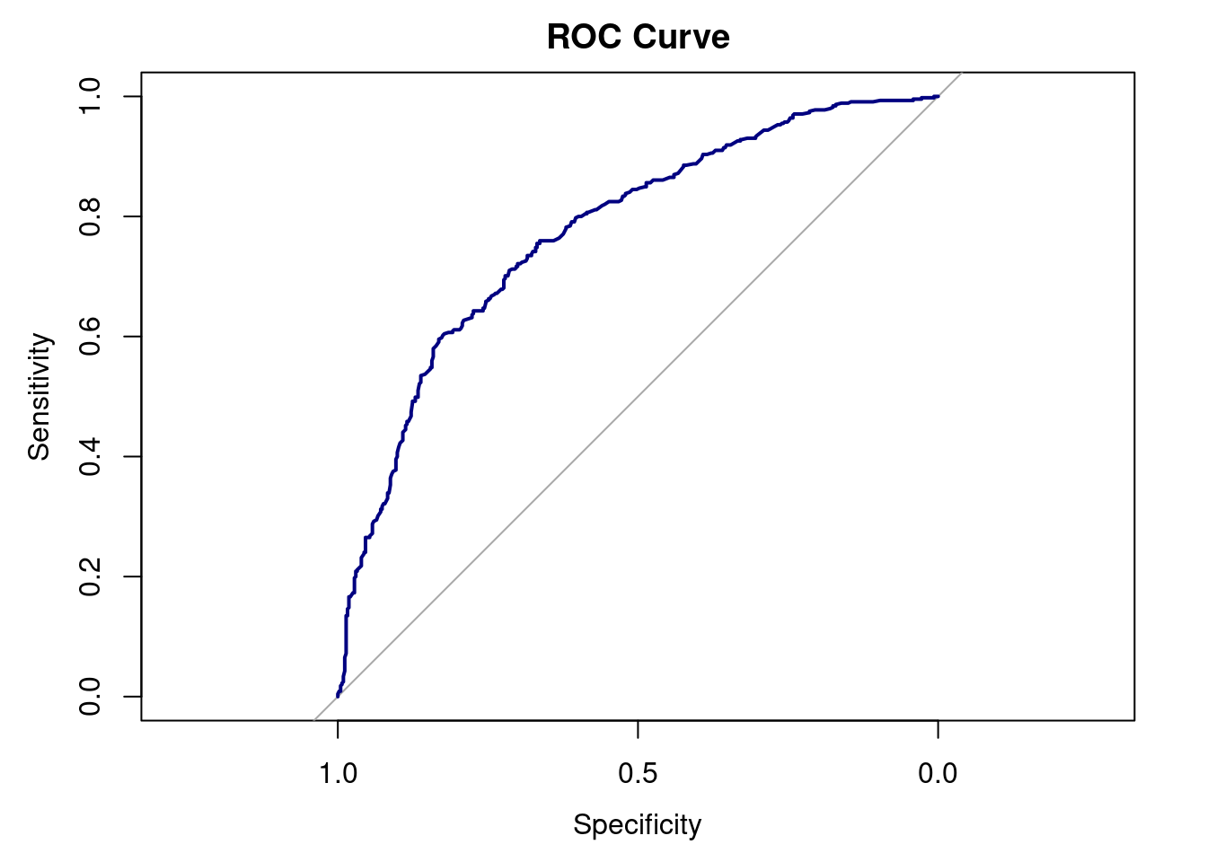
8.7.0.1 Model Interpretation:
On the test data, the model performed moderately well overall. It achieved an accuracy of 0.71, which is noticeably higher than the No Information Rate of 0.51, meaning the model performs better than simply predicting the most common wage category. The model also did a reasonable job identifying high earners, with a sensitivity of 0.72, and it correctly identified low earners at a similar rate (specificity = 0.70). These values produce a balanced accuracy of 0.71, suggesting the model performs consistently across both wage groups.
8.7.0.1.1 ROC Interpretation:
The ROC analysis produced an AUC of 0.77, suggesting that the model does a reasonably good job ranking individuals by their likelihood of being high earners, even if its classification accuracy is not perfect. Overall, the model shows moderate predictive performance on unseen data and provides informative probability estimates, although there remains room for improvement in how well it separates high and low earners.
8.8 Final Interpretation
In this analysis, we examined how age, education, job class, and marital status relate to wage levels by conducting classical statistical tests and building a predictive logistic regression model. The results from earlier analyses showed meaningful differences across several variables. Age differed significantly between high and low wage earners, with high earners being older on average. Education also showed large differences in wage, with higher levels of education generally associated with higher wages. Job class displayed additional variation in wage patterns, as industrial and information workers had different wage distributions. Marital status was also related to wage in the chi-square analysis, indicating that the distribution of high and low wage earners differed across marital groups.
The logistic regression analysis identified age and education as significant predictors of earning a high wage, while job class was not statistically significant in the model. Education showed the strongest effects, with individuals holding a high school diploma, some college, a college degree, or an advanced degree having substantially higher odds of being classified as high earners compared to those with less than a high school education. Age also influenced wage category, with older individuals showing slightly lower odds of being high earners. Job class showed only a modest difference between information and industrial workers, and this effect was not statistically reliable. Marital status was included in the dataset but was not used in the logistic regression model. Overall, education played the most prominent role in predicting wage level in this sample.
When the model was evaluated on unseen test data, its classification performance was moderate. The accuracy was 0.71, which is higher than the No Information Rate of 0.51, meaning that the model performs better than simply guessing the most common wage category. Sensitivity (0.72) and specificity (0.70) were both fairly similar, showing that the model identifies high and low earners about the same rate. The AUC value of 0.77 suggests that the model’s predicted probabilities do a reasonably good job ranking individuals from lower to higher likelihood of being high earners. Overall, the model works reasonably well on the test data and provides helpful probability estimates, but its classification accuracy could be better.
Lastly, the model predicted high and low earners at similar rates, with sensitivity (0.72) and specificity (0.70) showing that it identified both groups moderately well. Although marital status was significantly related to wage category in the chi-square test, it was not included in the logistic regression model because the focus was on age, education, and job class as predictors. If I were to repeat the analysis, I would consider testing whether marital status adds meaningful predictive value when included in the model. I would also consider adding additional predictors, such as region and health to further improve model accuracy.