library(tidyverse)
library(httr)
library(jsonlite)
library(supernova)
library(AICcmodavg)
library(mosaic)3 Law Firm Analysis
3.1 Introduction
In this chapter, we act as data scientists working for a law firm that specializes in fighting parking and camera tickets. The goal of this analysis is to uncover patterns in NYC violation data in order to better understand trends across different aspects of ticketing and inform the firm’s marketing strategy. Using the Open Parking and Camera Violations Data from NYC Open Data, we explore whether payment amounts differ by issuing agency, plate state, and county. To answer these questions, we use data cleaning, visualization with ggplot2, descriptive statistics, and one-way ANOVA to assess whether observed differences are statistically meaningful.
NoteIn this analysis we explore three questions:
Do certain agencies issue higher payments?
Do drivers from different states (NY, NJ, CT) pay more?
Do certain counties tend to have higher payment amounts?
3.2 Required Packages
First, we load the packages used in this report.
3.3 Data Ingestion via API
Next, we pull the Open Parking and Camera Violations data directly from NYC Open Data using httr::GET() and the endpoint below.
endpoint<-"https://data.cityofnewyork.us/resource/nc67-uf89.json"

resp <- httr::GET(endpoint, query = list(
  "$limit" = 99999,
  "$order" = "issue_date DESC"
))

camera <- jsonlite::fromJSON(httr::content(resp, as = "text"), flatten = TRUE)
3.4 Cleaning Data
Now that the dataset was successfully loaded, we began the data cleaning process.
camera<- camera %>%
  mutate(payment_amount = as.numeric(payment_amount))
We first converted the payment_amount variable from character to numeric so it could be used for statistical analysis.
camera <- camera %>% mutate(county=recode(county,
                                          "K"="Kings County",
                                          "BK"="Kings County",
                                          "Kings"="Kings County",
                                          "Kings Count"="Kings County",
                                          "Bronx"="Kings County",
                                          "Q"="Queens County",
                                          "QN"="Queens County",
                                          "Qns"="Queens County",
                                          "BX"="Bronx County",
                                          "NY"="New York County",
                                          "MN"="New York County",
                                          "R"="Richmond County",
                                          "RICH"="Richmond County",
                                          "ST"="Richmond County"))
We also recoded county abbreviations into their full county names to improve clarity and consistency.
3.5 Payment Amount by Agency
3.5.1 Visualization
ggplot(camera, aes(x = issuing_agency, y = payment_amount)) +
  geom_boxplot() +
  theme_minimal() +
  coord_flip() +
  labs(
    title = "Payment Amount by Agency",
    x = "Agency",
    y = "Payment Amount ($)"
  )
Warning: Removed 65 rows containing non-finite outside the scale range
(`stat_boxplot()`).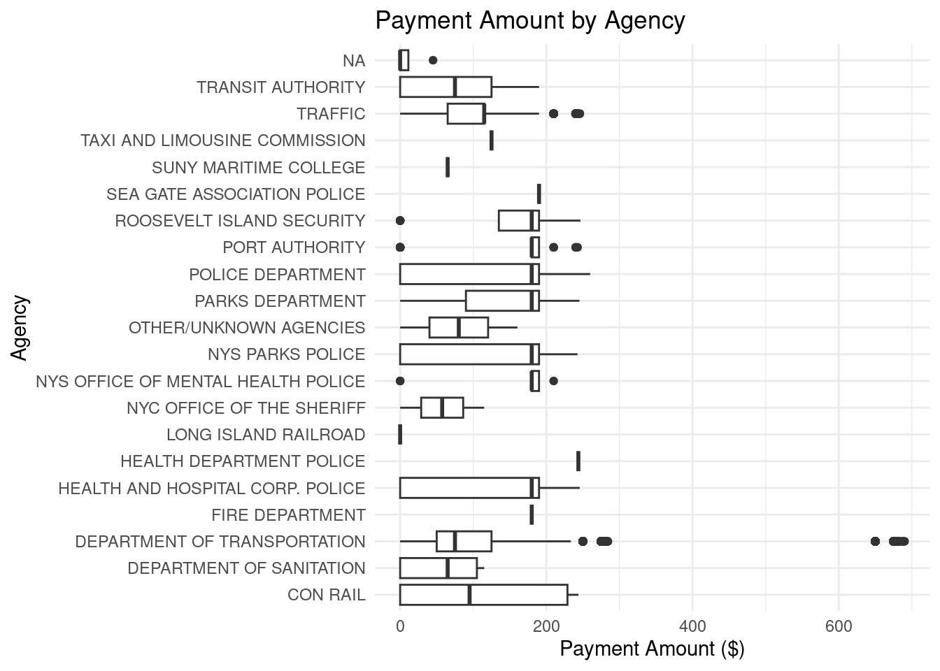
3.5.2 Descriptive Statistics
favstats(payment_amount ~ issuing_agency, data = camera) %>% arrange(desc(mean)) issuing_agency min Q1 median Q3 max
1 HEALTH DEPARTMENT POLICE 243.81 243.810 243.81 243.8100 243.81
2 SEA GATE ASSOCIATION POLICE 190.00 190.000 190.00 190.0000 190.00
3 FIRE DEPARTMENT 180.00 180.000 180.00 180.0000 180.00
4 NYS OFFICE OF MENTAL HEALTH POLICE 0.00 180.000 180.00 190.0000 210.00
5 ROOSEVELT ISLAND SECURITY 0.00 135.000 180.00 190.0000 246.68
6 PORT AUTHORITY 0.00 180.000 180.00 190.0000 242.76
7 NYS PARKS POLICE 0.00 0.000 180.00 190.0000 242.58
8 PARKS DEPARTMENT 0.00 90.000 180.00 190.0000 245.28
9 TAXI AND LIMOUSINE COMMISSION 125.00 125.000 125.00 125.0000 125.00
10 HEALTH AND HOSPITAL CORP. POLICE 0.00 0.000 180.00 190.0000 245.64
11 POLICE DEPARTMENT 0.00 0.000 180.00 190.0000 260.00
12 CON RAIL 0.00 0.000 95.00 228.8875 243.87
13 DEPARTMENT OF TRANSPORTATION 0.00 50.000 75.00 125.0000 690.04
14 TRAFFIC 0.00 65.000 115.00 115.0000 245.79
15 OTHER/UNKNOWN AGENCIES 0.00 40.115 80.23 120.3450 160.46
16 TRANSIT AUTHORITY 0.00 0.000 75.00 125.0000 190.00
17 SUNY MARITIME COLLEGE 65.00 65.000 65.00 65.0000 65.00
18 NYC OFFICE OF THE SHERIFF 0.00 28.750 57.50 86.2500 115.00
19 DEPARTMENT OF SANITATION 0.00 0.000 65.00 105.0000 115.00
20 LONG ISLAND RAILROAD 0.00 0.000 0.00 0.0000 0.00
mean sd n missing
1 243.81000 NA 1 0
2 190.00000 0.00000 2 0
3 180.00000 NA 1 0
4 161.33333 65.99423 15 0
5 149.16083 90.57967 24 0
6 147.35792 82.58394 48 0
7 139.75143 91.22029 35 0
8 128.47736 78.92728 144 0
9 125.00000 NA 1 0
10 124.71373 98.60130 51 0
11 123.93855 88.00388 214 0
12 112.62000 124.87146 6 0
13 99.52878 82.88425 87272 0
14 94.59362 44.47453 12091 0
15 80.23000 113.46235 2 0
16 78.00000 82.05181 5 0
17 65.00000 NA 1 0
18 57.50000 81.31728 2 0
19 56.78571 48.26239 14 0
20 0.00000 NA 1 03.5.3 Inferential Statistics
anova_agency <- aov(payment_amount ~ issuing_agency, data = camera)
summary(anova_agency)
Df Sum Sq Mean Sq F value Pr(>F)
issuing_agency 19 927433 48812 7.772 <2e-16 ***
Residuals 99910 627482336 6280
---
Signif. codes: 0 '***' 0.001 '**' 0.01 '*' 0.05 '.' 0.1 ' ' 1
69 observations deleted due to missingnesssupernova(anova_agency)Refitting to remove 69 cases with missing value(s)
ℹ aov(formula = payment_amount ~ issuing_agency, data = listwise_delete(camera,
c("payment_amount", "issuing_agency"))) Analysis of Variance Table (Type III SS)
Model: payment_amount ~ issuing_agency
SS df MS F PRE p
----- --------------- | ------------- ----- --------- ----- ----- -----
Model (error reduced) | 927432.864 19 48812.256 7.772 .0015 .0000
Error (from model) | 627482335.766 99910 6280.476
----- --------------- | ------------- ----- --------- ----- ----- -----
Total (empty model) | 628409768.630 99929 6288.563 The ANOVA results show that the Sum of Squares for issuing_agency (SS = 927,432.864) is much smaller than the Residuals (SS = 627,482,335.765), meaning agency explains very little of the variance in payment_amount. The F value of 7.77 and very low p-value (< .001) indicate a statistically significant difference between agencies, but the PRE value (0.0015) shows that agency explains only about 0.15% of the variance. In other words, the result is statistically significant but too small to matter in real-world terms.
3.5.4 Interpretation
The results show that while there are some differences in payment amounts between agencies, the difference is very small. Even though the test came out statistically significant, the actual effect isn’t meaningful in the real world. This suggests that the type of agency has very little influence on how much people end up paying. So, I would not recommend the law firm focus on agency as part of their marketing strategy since it doesn’t seem to have a big impact.
3.6 Payment Amount by Tri-State (NY, NJ, CT)
3.6.1 Visualization
camera_tri <- camera %>% filter(state %in% c("NY","NJ","CT"))

#plate_state x payment_amount
ggplot(camera_tri, aes(x = state, y = payment_amount)) +
  geom_boxplot() +
  theme_minimal() +
  coord_flip() +
  labs(
    title = "Payment Amount by State",
    x = "State",
    y = "Payment Amount ($)"
  )
Warning: Removed 15 rows containing non-finite outside the scale range
(`stat_boxplot()`).
3.6.2 Descriptive Statistics
favstats(payment_amount ~ state, data = camera_tri) %>% arrange(desc(mean)) state min Q1 median Q3 max mean sd n missing
1 NJ 0 50 75 115 682.35 101.5746 89.97170 8654 3
2 NY 0 50 75 125 690.04 101.0908 80.93045 79540 10
3 CT 0 50 75 100 276.57 80.6627 46.07849 1457 23.6.3 Inferential Statistics
anova_state <- aov(payment_amount ~ state, data = camera_tri)
summary(anova_state)
Df Sum Sq Mean Sq F value Pr(>F)
state 2 602745 301373 45.48 <2e-16 ***
Residuals 89648 594096287 6627
---
Signif. codes: 0 '***' 0.001 '**' 0.01 '*' 0.05 '.' 0.1 ' ' 1
15 observations deleted due to missingnesssupernova(anova_state)Refitting to remove 15 cases with missing value(s)
ℹ aov(formula = payment_amount ~ state, data = listwise_delete(camera_tri,
c("payment_amount", "state"))) Analysis of Variance Table (Type III SS)
Model: payment_amount ~ state
SS df MS F PRE p
----- --------------- | ------------- ----- ---------- ------ ----- -----
Model (error reduced) | 602745.209 2 301372.604 45.477 .0010 .0000
Error (from model) | 594096286.652 89648 6626.989
----- --------------- | ------------- ----- ---------- ------ ----- -----
Total (empty model) | 594699031.861 89650 6633.564 The ANOVA results show that the Sum of Squares for state (SS = 602,745.209) is much smaller than the residual variance (SS = 594,096,286.652), indicating that state accounts for only a very small portion of the variation in payment_amount. The F statistic of 45.48 with a very low p-value (p < .001) indicates a statistically significant difference in payment amounts between states. However, the PRE value (.0010) shows that state explains only about 0.1% of the variance. This suggests that although there is a statistical difference across NY, NJ, and CT, the effect is extremely small and not practically meaningful.
3.6.4 Interpretation
The results show that there are some differences in payment amounts between New York, New Jersey, and Connecticut, but the differences are very small. Even though the test came out statistically significant, it doesn’t make a real impact in the real world. The state someone is from doesn’t seem to strongly affect how much they pay for their tickets. As a result, I would not recommend the law firm use state as a focus in their marketing strategy since it doesn’t seem to be an important factor.
3.7 Payment Amount by County
3.7.1 Visualization
ggplot(camera, aes(x = county, y = payment_amount)) +
  geom_boxplot() +
  theme_minimal() +
  coord_flip() +
  labs(
    title = "Payment Amount by County",
    x = "County",
    y = "Payment Amount ($)"
  )
Warning: Removed 65 rows containing non-finite outside the scale range
(`stat_boxplot()`).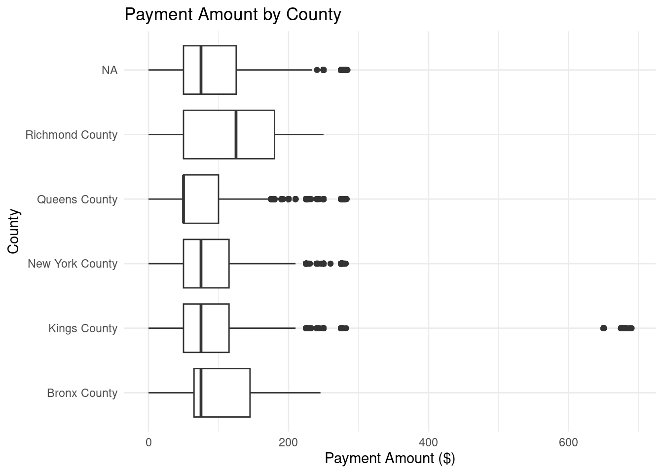
3.7.2 Descriptive Statistics
favstats(payment_amount ~ county, data = camera) %>% arrange(desc(mean)) county min Q1 median Q3 max mean sd n missing
1 Richmond County 0 50 125 180 250.00 114.53669 77.55385 1349 0
2 Kings County 0 50 75 115 690.04 110.89009 126.20057 16113 0
3 Bronx County 0 65 75 145 245.64 99.59634 67.66429 246 0
4 New York County 0 50 75 115 281.80 97.62502 62.55866 23479 0
5 Queens County 0 50 50 100 283.03 83.46501 60.08515 17366 03.7.3 Inferential Statistics
anova_county <- aov(payment_amount ~ county, data = camera)
summary(anova_county)
Df Sum Sq Mean Sq F value Pr(>F)
county 4 6702697 1675674 233.4 <2e-16 ***
Residuals 58548 420413252 7181
---
Signif. codes: 0 '***' 0.001 '**' 0.01 '*' 0.05 '.' 0.1 ' ' 1
41446 observations deleted due to missingnesssupernova(anova_county)Refitting to remove 41446 cases with missing value(s)
ℹ aov(formula = payment_amount ~ county, data = listwise_delete(camera,
c("payment_amount", "county"))) Analysis of Variance Table (Type III SS)
Model: payment_amount ~ county
SS df MS F PRE p
----- --------------- | ------------- ----- ----------- ------- ----- -----
Model (error reduced) | 6702697.176 4 1675674.294 233.359 .0157 .0000
Error (from model) | 420413251.683 58548 7180.659
----- --------------- | ------------- ----- ----------- ------- ----- -----
Total (empty model) | 427115948.859 58552 7294.643 The ANOVA results show that the Sum of Squares for county (SS = 6,702,697.176) is small compared to the residual variance (SS = 420,413,251.683), meaning that county explains only a small portion of the total variation in payment_amount. The Mean Square for county is higher than the residual Mean Square, indicating that there are differences in payment amounts between counties. The F value of 233.36 is very large, and the very small p-value (p < .001) shows that these differences are statistically significant. However, the PRE value (.0157) indicates that only about 1.57% of the total variance in payment_amount is explained by county. This means that while the result is statistically significant, the actual differences in payment amounts between counties are still small and not practically meaningful.
3.7.4 Interpretation
Again, the results show that while payment amounts vary slightly across different counties, the differences are very small overall. Even though the analysis was statistically significant, it doesn’t make a real-world impact. This suggests that the county where a ticket is issued doesn’t strongly affect how much people pay. Therefore, I would not recommend the law firm focus on county differences in their marketing strategy either, since it’s not an important factor influencing payment amounts.
3.8 Concluding Summary
After comparing payment amounts by agency, state, and county, none of the variables really stood out as being meaningful in explaining differences in payment amounts. While all three tests were statistically significant, the actual differences were very small in real-world terms. This means that factors like agency type, state, or county don’t seem to strongly influence how much people pay for their tickets. For that reason, I wouldn’t recommend the firm focus on any of these variables for marketing purposes. Instead, it may be more useful to explore other factors, like the type of vehicle, which might be a better predictor of higher payments.
ImportantKey Takeaway
Even though the results were statistically significant, the actual differences were very small. This shows why it’s important not to rely only on p-values. Looking at effect size helped me see that these variables don’t meaningfully explain payment differences in practice.