library(tidyverse)
library(readxl)
library(dplyr)
library(stringr)
library(knitr)
library(ggplot2)
library(ggpubr)
library(ggcorrplot)
library(AICcmodavg)
library(broom)6 Florida Crime Analytics
6.1 Introduction
In this report, we analyze county-level crime data in Florida to explore the relationship between crime rates and important socioeconomic factors. Specifically, we look at how crime relates to median income, high school graduation rates, and urban population, and determine which of these variables best predicts county-level crime rates across the state.
6.2 Required Packages
First, we load the packages used in this report.
6.3 Loading and Preparing the Data
florida_crime <- read_xlsx("Florida County Crime Rates.xlsx")

florida_crime <- florida_crime %>%
  rename(Crime = C,
         Income = I,
         HighSchoolGrad = HS,
         UrbanPop = U) %>%
  mutate(County = str_to_title(tolower(County)))

summary(florida_crime)
County Crime Income HighSchoolGrad
Length:67 Min. : 0.0 Min. :15.40 Min. :54.50
Class :character 1st Qu.: 35.5 1st Qu.:21.05 1st Qu.:62.45
Mode :character Median : 52.0 Median :24.60 Median :69.00
Mean : 52.4 Mean :24.51 Mean :69.49
3rd Qu.: 69.0 3rd Qu.:28.15 3rd Qu.:76.90
Max. :128.0 Max. :35.60 Max. :84.90
UrbanPop
Min. : 0.00
1st Qu.:21.60
Median :44.60
Mean :49.56
3rd Qu.:83.55
Max. :99.60 First, we loaded the dataset from Excel, renamed the columns to standardize them (Crime, Income, HighSchoolGrad, UrbanPop), and reformatted the county names so only the first letter is capitalized for consistency. Then, we used summary() to get a general overview of the dataset.
6.4 Exploratory Data Analysis
6.4.1 Basic descriptive statistics (mean, median, range)
descriptive_stats <- data.frame(
  Statistic = c("Mean", "Median", "Range"),
  Crime = c(mean(florida_crime$Crime),
            median(florida_crime$Crime),
            diff(range(florida_crime$Crime))),
  Income = c(mean(florida_crime$Income),
             median(florida_crime$Income),
             diff(range(florida_crime$Income))),
  HighSchoolGrad = c(mean(florida_crime$HighSchoolGrad),
                     median(florida_crime$HighSchoolGrad),
                     diff(range(florida_crime$HighSchoolGrad))),
  UrbanPop = c(mean(florida_crime$UrbanPop),
               median(florida_crime$UrbanPop),
               diff(range(florida_crime$UrbanPop))))

knitr::kable(descriptive_stats) | Statistic | Crime | Income | HighSchoolGrad | UrbanPop |
|---|---|---|---|---|
| Mean | 52.40299 | 24.51045 | 69.48955 | 49.55821 |
| Median | 52.00000 | 24.60000 | 69.00000 | 44.60000 |
| Range | 128.00000 | 20.20000 | 30.40000 | 99.60000 |
Then, we calculated basic descriptive statistics (mean, median, and range) for all numeric variables in the dataset — Crime, Income, HighSchoolGrad, and UrbanPop and organized the results into a table for easier comparison.
6.4.2 Scatterplot: Median income (in thousands) + Crime rate (per 1,000 residents)
ggplot(florida_crime, aes(x = Income, y = Crime)) +
  geom_point (size = 3) +
  geom_smooth(method = "lm", se = FALSE) +
  stat_cor(method = "pearson") +
  labs(title = "Relationship Between Crime rate and Median income",
       x = "Median income (in thousands)",
       y = "Crime rate (per 1,000 residents)") +
  theme_minimal(base_size = 12) +
  theme(plot.title = element_text(size = 17, family = "Georgia", face = "bold"),
        axis.title.x = element_text(size = 12, family = "Georgia"),
        axis.title.y = element_text(size = 12, family = "Georgia"))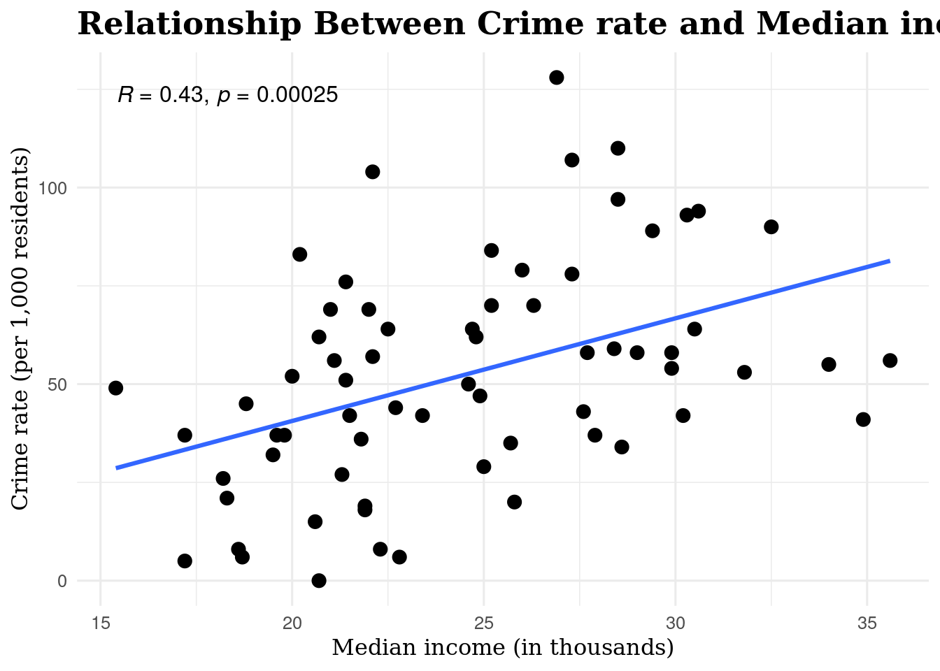
6.4.2.1 Interpretation:
The scatter plot shows a moderate positive relationship between median income and crime rate (r ≈ 0.43). As income increases, crime rates also tend to rise slightly, although there is still some variation.
6.4.3 Scatterplot: Urban population (%) + Crime rate (per 1,000 residents)
ggplot(florida_crime, aes(x = UrbanPop, y = Crime)) +
  geom_point (size = 3) +
  geom_smooth(method = "lm", se = FALSE) +
  stat_cor(method = "pearson") +
  labs(title = "Relationship Between Crime rate and Urban population",
       x = "Urban population (%)",
       y = "Crime rate (per 1,000 residents)") +
  theme_minimal(base_size = 12) +
  theme(plot.title = element_text(size = 17, family = "serif", face = "bold"),
        axis.title.x = element_text(size = 12, family = "serif"),
        axis.title.y = element_text(size = 12, family = "serif"))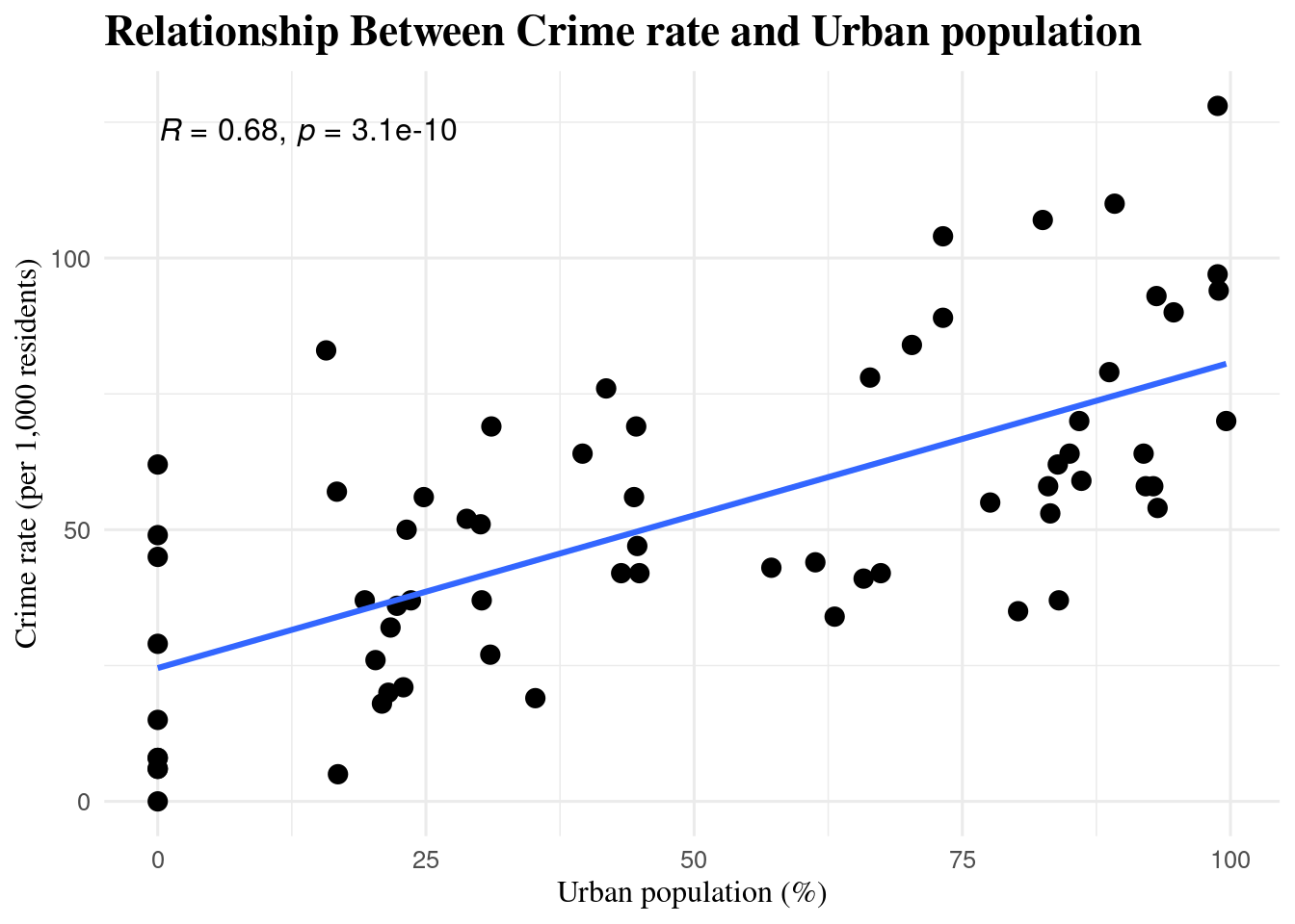
6.4.3.1 Interpretation:
The scatter plot shows a fairly strong positive relationship between urban population percentage and crime rate (r ≈ 0.68). This suggests that counties with a larger urban population tend to have higher crime rates. The trend line supports this pattern.
6.5 Correlation Analysis
6.5.1 Correlation matrix:
cor_matrix <- cor(florida_crime[,c("Crime","Income","HighSchoolGrad","UrbanPop")])
cor_matrix
Crime Income HighSchoolGrad UrbanPop
Crime 1.0000000 0.4337503 0.4669119 0.6773678
Income 0.4337503 1.0000000 0.7926215 0.7306983
HighSchoolGrad 0.4669119 0.7926215 1.0000000 0.7907190
UrbanPop 0.6773678 0.7306983 0.7907190 1.00000006.5.2 Visualization:
ggcorrplot(cor_matrix,
           lab = TRUE,
           title = "Correlation Matrix: Crime, Income, HighSchoolGrad, UrbanPop",
           lab_size = 3,
           colors=)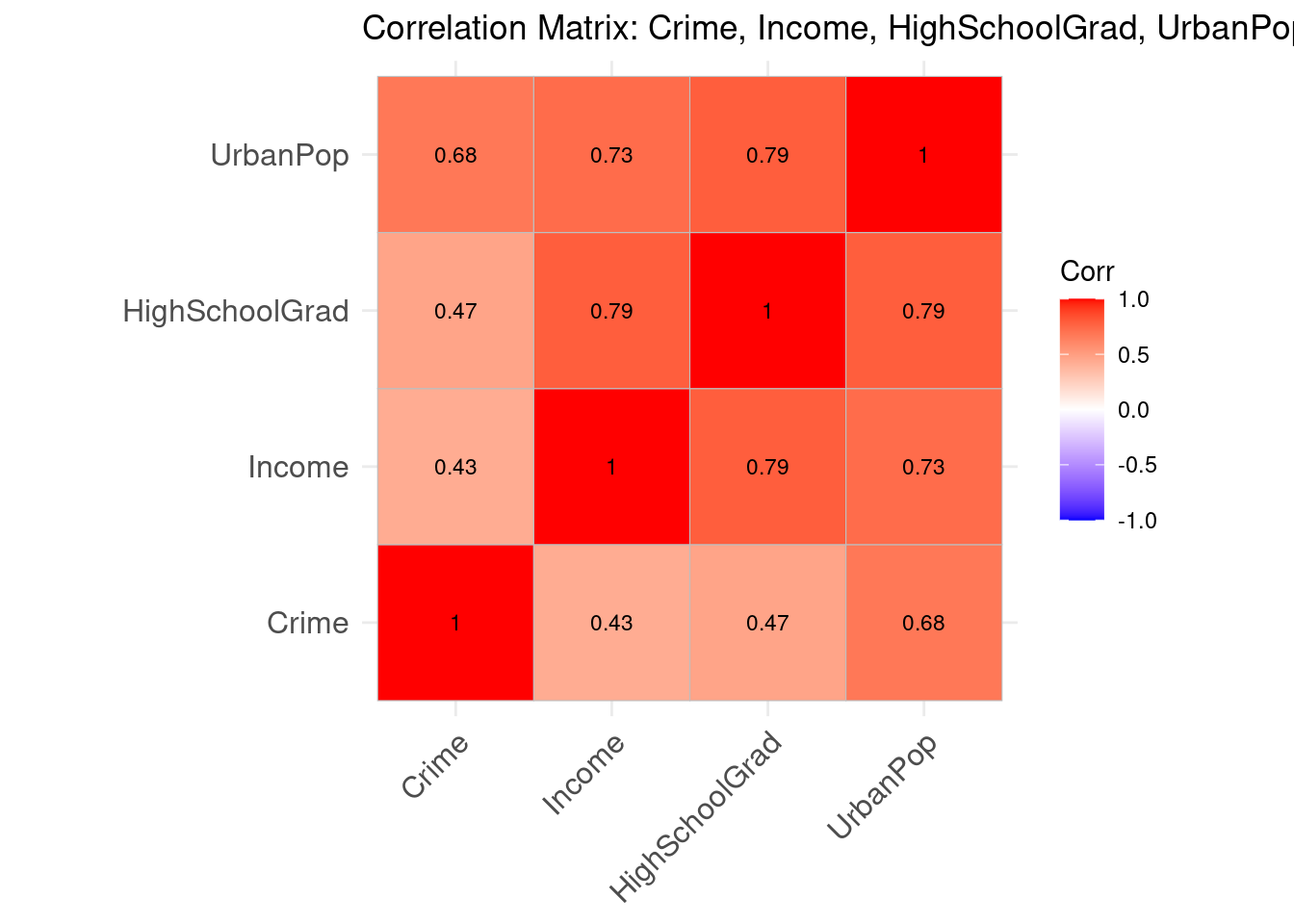
6.5.2.1 Interpretation:
All variables show a positive relationship with crime. Income (r ≈ 0.43) and high school graduation rate (r ≈ 0.47) have moderate positive correlations, while urban population (r ≈ 0.68) shows a strong positive correlation and is the strongest predictor of crime out of the variables.
6.6 Building Regression Models
6.6.1 Building a simple regression model:
model_income <- lm(Crime ~ Income, data = florida_crime)
summary(model_income)
Call:
lm(formula = Crime ~ Income, data = florida_crime)

Residuals:
    Min      1Q  Median      3Q     Max
-42.452 -21.347  -3.102  17.580  69.357

Coefficients:
            Estimate Std. Error t value Pr(>|t|)
(Intercept) -11.6059    16.7863  -0.691 0.491782
Income        2.6115     0.6729   3.881 0.000246 ***
---
Signif. codes:  0 '***' 0.001 '**' 0.01 '*' 0.05 '.' 0.1 ' ' 1

Residual standard error: 25.6 on 65 degrees of freedom
Multiple R-squared:  0.1881,    Adjusted R-squared:  0.1756
F-statistic: 15.06 on 1 and 65 DF,  p-value: 0.0002456
6.6.2 Building multiple regression models:
model_income_highschoolgrad <- lm(Crime ~ Income + HighSchoolGrad, data = florida_crime)
model_income_urbanpop <- lm(Crime ~ Income + UrbanPop, data = florida_crime)
model_all <- lm(Crime ~ Income + HighSchoolGrad + UrbanPop, data = florida_crime)

summary(model_income_highschoolgrad)
Call:
lm(formula = Crime ~ Income + HighSchoolGrad, data = florida_crime)

Residuals:
   Min     1Q Median     3Q    Max
-42.75 -19.61  -4.57  18.52  77.86

Coefficients:
               Estimate Std. Error t value Pr(>|t|)
(Intercept)    -46.1094    24.9723  -1.846   0.0695 .
Income           1.0311     1.0839   0.951   0.3450
HighSchoolGrad   1.0540     0.5729   1.840   0.0705 .
---
Signif. codes:  0 '***' 0.001 '**' 0.01 '*' 0.05 '.' 0.1 ' ' 1

Residual standard error: 25.14 on 64 degrees of freedom
Multiple R-squared:  0.2289,    Adjusted R-squared:  0.2048
F-statistic: 9.5 on 2 and 64 DF, p-value: 0.000244summary(model_income_urbanpop)
Call:
lm(formula = Crime ~ Income + UrbanPop, data = florida_crime)

Residuals:
    Min      1Q  Median      3Q     Max
-36.130 -15.590  -6.484  16.595  48.921

Coefficients:
            Estimate Std. Error t value Pr(>|t|)
(Intercept)  39.9723    16.3536   2.444   0.0173 *
Income       -0.7906     0.8049  -0.982   0.3297
UrbanPop      0.6418     0.1110   5.784 2.36e-07 ***
---
Signif. codes:  0 '***' 0.001 '**' 0.01 '*' 0.05 '.' 0.1 ' ' 1

Residual standard error: 20.91 on 64 degrees of freedom
Multiple R-squared:  0.4669,    Adjusted R-squared:  0.4502
F-statistic: 28.02 on 2 and 64 DF, p-value: 1.815e-09summary(model_all)
Call:
lm(formula = Crime ~ Income + HighSchoolGrad + UrbanPop, data = florida_crime)

Residuals:
    Min      1Q  Median      3Q     Max
-35.407 -15.080  -6.588  16.178  50.125

Coefficients:
               Estimate Std. Error t value Pr(>|t|)
(Intercept)     59.7147    28.5895   2.089   0.0408 *
Income          -0.3831     0.9405  -0.407   0.6852
HighSchoolGrad  -0.4673     0.5544  -0.843   0.4025
UrbanPop         0.6972     0.1291   5.399 1.08e-06 ***
---
Signif. codes:  0 '***' 0.001 '**' 0.01 '*' 0.05 '.' 0.1 ' ' 1

Residual standard error: 20.95 on 63 degrees of freedom
Multiple R-squared:  0.4728,    Adjusted R-squared:  0.4477
F-statistic: 18.83 on 3 and 63 DF,  p-value: 7.823e-09
6.6.3 Comparing R², Adjusted R², AIC values:
AIC(model_income, model_income_highschoolgrad, model_income_urbanpop, model_all) %>%
  as.data.frame() %>%
  dplyr::arrange(AIC)
df AIC
model_income_urbanpop 4 602.4276
model_all 5 603.6764
model_income_highschoolgrad 4 627.1524
model_income 3 628.6045models <- list(model_income, model_income_highschoolgrad, model_income_urbanpop,model_all)
names(models) <- c("model_income", "model_income_highschoolgrad", "model_income_urbanpop",
"model_all")
purrr::map_dfr(models, broom::glance, .id = "model") %>%
dplyr::select(model, r.squared, adj.r.squared, p.value, AIC)# A tibble: 4 × 5
model r.squared adj.r.squared p.value AIC
<chr> <dbl> <dbl> <dbl> <dbl>
1 model_income 0.188 0.176 0.000246 629.
2 model_income_highschoolgrad 0.229 0.205 0.000244 627.
3 model_income_urbanpop 0.467 0.450 0.00000000181 602.
4 model_all 0.473 0.448 0.00000000782 604.6.6.3.1 Interpretation:
When comparing models, the one with Income and UrbanPop (model_income_urbanpop) has the lowest AIC (602), meaning it provides the best balance between accuracy and simplicity. It also has a relatively high adjusted R² (0.45), showing it explains a good portion of the variance in crime without unnecessary complexity. The full model (adding HighSchoolGrad) has a slightly lower adjusted R² (0.448) and a higher AIC (604), indicating that adding HighSchoolGrad does not meaningfully improve the model. Therefore, UrbanPop appears to be the most influential predictor, and the model with Income + UrbanPop is the best overall in terms of simplicity and predictive performance.
6.6.3.2 Therefore,
counties with larger urban populations tend to have higher crime rates. For every 1% increase in the urban population, the predicted crime rate increases by about 0.56 incidents per 1,000 residents, holding income constant. This relationship is positive, moderately strong (adjusted R² ≈ 0.45), and statistically significant (p < 0.001). This suggests that more urbanized areas in Florida experience higher crime, possibly due to greater population density or urban conditions.
ImportantKey Finding
The model that best predicts county-level crime rates includes both median income and urban population. Together, these variables explain a substantial portion of the variation in crime across counties (Adjusted R² ≈ 0.45) while maintaining model simplicity. Among them, urban population is the strongest individual predictor, showing the highest correlation with crime and remaining significant across models.
6.7 Communicating Findings
After looking at the Florida county crime data, we found that the model that predicts crime the best includes both median income and urban population. This model explains about 45% of the differences in crime rates across counties (Adjusted R² ≈ 0.45) and also has the lowest AIC, meaning it fits well without being too complex. Urban population turned out to be the strongest predictor, it has the highest correlation with crime (r ≈ 0.68) and stays significant in every model. Ultimately, this means that counties with more people living in urban areas tend to have higher crime rates. Because of this, it might make sense for the Florida Police Department to focus more resources and prevention in highly urban counties. One limitation is that, like any correlation analysis, it does not prove causation. Additionally, this model does not account for other important socioeconomic factors, such as unemployment or poverty, which could also influence crime rates.
6.8 Final Comment
Lastly, based on our analysis, the model that best predicts Florida’s county-level crime rates is the one using both median income and urban population (Crime ~ Income + UrbanPop). This model has the lowest AIC and is able to explain almost half of the differences in crime rates between counties. Urban population is the strongest predictor, and income slightly improves the model’s accuracy, making this combination the most effective for understanding crime differences across counties.