library(tidyverse)
library(lubridate)
library(stringr)
library(tidyr)
library(ggplot2)
library(dplyr)
library(knitr)
library(readr)
library(janitor)2 Introduction to R Markdown
2.1 Introduction
In this chapter, we turn an R script into a fully reproducible R Markdown report using the NYPD Shooting Incident Data from NYC Open Data. We load the dataset through an API, clean and prepare the data, explore patterns, and create tables and visualizations using kable() and ggplot2. The goal is to practice building a clear, reproducible workflow that combines code, narrative text, and results in a single document.
2.2 Required Packages
First, we load the packages used in this report.
WarningNote about the dataset source
The NYPD Shooting Incident dataset used in the original assignment is no longer available through the NYC Open Data API. To keep this chapter reproducible, we use the CSV version of the dataset provided in class instead.
2.3 Data Ingestion (CSV substitute)
Next, we load the NYPD shooting incident data from the CSV file provided for this assignment, which serves as a substitute for the original NYC Open Data API source.
shooting_data <- read_csv("NYPD_Shooting_Incident_Data__Historic__20250910.csv")Rows: 29744 Columns: 21
── Column specification ────────────────────────────────────────────────────────
Delimiter: ","
chr (12): OCCUR_DATE, BORO, LOC_OF_OCCUR_DESC, LOC_CLASSFCTN_DESC, LOCATION...
dbl (5): INCIDENT_KEY, PRECINCT, JURISDICTION_CODE, Latitude, Longitude
num (2): X_COORD_CD, Y_COORD_CD
lgl (1): STATISTICAL_MURDER_FLAG
time (1): OCCUR_TIME
ℹ Use `spec()` to retrieve the full column specification for this data.
ℹ Specify the column types or set `show_col_types = FALSE` to quiet this message.
NoteExample API Code
Although the analysis uses a CSV file due to the API being unavailable, the code below demonstrates how the dataset would normally be retrieved using the NYC Open Data API.
# Using an API to call the data ####
endpoint <- "https://data.cityofnewyork.us/resource/833y-fsy8.json"

# Example: get 5,000 most recent rows
resp <- GET(endpoint, query = list(
  "$limit" = 30000,
  "$order" = "OCCUR_DATE DESC"
))

# Parse JSON into R dataframe
shooting_data <- fromJSON(content(resp, as = "text"), flatten = TRUE)
The dataset includes incidents across a range of dates, from 01/01/2006 to 12/31/2024.
2.4 Cleaning Data
Now that the dataset was successfully loaded, we began the data cleaning process.
2.4.1 Removing NA rows in perp_race
# Check how many missing values each column has
colSums(is.na(shooting_data))
INCIDENT_KEY OCCUR_DATE OCCUR_TIME
0 0 0
BORO LOC_OF_OCCUR_DESC PRECINCT
0 25596 0
JURISDICTION_CODE LOC_CLASSFCTN_DESC LOCATION_DESC
2 25596 14977
STATISTICAL_MURDER_FLAG PERP_AGE_GROUP PERP_SEX
0 9344 9310
PERP_RACE VIC_AGE_GROUP VIC_SEX
9310 0 0
VIC_RACE X_COORD_CD Y_COORD_CD
0 0 0
Latitude Longitude Lon_Lat
97 97 97 # Standardize column names
shooting_data <- shooting_data %>% clean_names()
# Check missing values specifically in perp_race
sum(is.na(shooting_data$perp_race))[1] 9310# Remove rows where perp_race is missing or marked as unavailable
shooting_clean<-shooting_data %>% filter(
!is.na(perp_race) &
!(perp_race %in% c("(NULL)","UNKNOWN","(null)")))
# Confirm that missing values were removed
sum(is.na(shooting_clean$perp_race))[1] 0Here, we check how many missing values are present across the dataset. We then focus on the perp_race column, which originally contains 9310 missing values. After filtering out rows with missing or unavailable values, we check the column again to confirm that the cleaning step is successful.
2.4.2 Making perp_race Values Lowercase
Next, we standardize the perp_race column by converting all values to lowercase. This prevents duplicate categories that differ only by capitalization.
shooting_clean<-shooting_clean %>% mutate(
  perp_race=str_to_lower(perp_race))
2.4.3 Creating a time_of_day Column
After some initial cleaning and standardizing, we now create a new column called time_of_day that groups each incident into broader time categories.
# Split occur_time into Hour, Minute, and Second
shooting_clean<- shooting_data %>% separate(
  col = occur_time,
  into = c("Hour","Minute","Second"),
  sep = ":",
)

# Create a time_of_day category based on the Hour value
shooting_clean <- shooting_clean %>% mutate(
  time_of_day = case_when(
    Hour < 12 ~ "Morning",
    Hour < 18 ~ "Afternoon",
    Hour >= 18 ~ "Night"
  ))
To create the time_of_day column, we first split the occur_time variable into separate Hour, Minute, and Second columns. Then we group the Hour values into three categories: Morning, Afternoon, and Night. The number of shootings in each group is ; Morning Afternoon Night ; 12466 5439 11839 .
2.5 Insights
2.5.1 Time of Day
Next, we summarize how often shootings occur during each time of day.
# View the names of the columns in the NYPD Shooting dataset
colnames(shooting_clean)
[1] "incident_key" "occur_date"
[3] "Hour" "Minute"
[5] "Second" "boro"
[7] "loc_of_occur_desc" "precinct"
[9] "jurisdiction_code" "loc_classfctn_desc"
[11] "location_desc" "statistical_murder_flag"
[13] "perp_age_group" "perp_sex"
[15] "perp_race" "vic_age_group"
[17] "vic_sex" "vic_race"
[19] "x_coord_cd" "y_coord_cd"
[21] "latitude" "longitude"
[23] "lon_lat" "time_of_day" # Count shootings by time of day in descending order
shooting_clean %>% count(time_of_day)%>% arrange(desc(n))# A tibble: 3 × 2
time_of_day n
<chr> <int>
1 Morning 12466
2 Night 11839
3 Afternoon 5439# Count shootings by time of day and borough in descending order
shooting_clean %>% count(time_of_day,boro) %>% arrange(desc(n))# A tibble: 15 × 3
time_of_day boro n
<chr> <chr> <int>
1 Night BROOKLYN 4737
2 Morning BROOKLYN 4610
3 Night BRONX 3672
4 Morning BRONX 3606
5 Afternoon BROOKLYN 2338
6 Morning QUEENS 2118
7 Morning MANHATTAN 1761
8 Night MANHATTAN 1596
9 Afternoon BRONX 1556
10 Night QUEENS 1529
11 Afternoon QUEENS 779
12 Afternoon MANHATTAN 620
13 Morning STATEN ISLAND 371
14 Night STATEN ISLAND 305
15 Afternoon STATEN ISLAND 146# Create a summary table with counts and percentages for each time of day category
time_summary <- shooting_clean %>%
filter(!is.na(time_of_day)) %>%
count(time_of_day, name = "n") %>%
mutate(pct = round(100 * n / sum(n), 1)) %>%
arrange(desc(n))
time_summary# A tibble: 3 × 3
time_of_day n pct
<chr> <int> <dbl>
1 Morning 12466 41.9
2 Night 11839 39.8
3 Afternoon 5439 18.3We count incidents in the Morning, Afternoon, and Night and arrange them from highest to lowest. The highest rate occurs during Morning (12466 cases; 41.9%).
2.5.2 Sex of Perpetrator
We also summarize the distribution of perpetrator sex.
# View the names of the columns in the NYPD Shooting dataset
colnames(shooting_clean)
[1] "incident_key" "occur_date"
[3] "Hour" "Minute"
[5] "Second" "boro"
[7] "loc_of_occur_desc" "precinct"
[9] "jurisdiction_code" "loc_classfctn_desc"
[11] "location_desc" "statistical_murder_flag"
[13] "perp_age_group" "perp_sex"
[15] "perp_race" "vic_age_group"
[17] "vic_sex" "vic_race"
[19] "x_coord_cd" "y_coord_cd"
[21] "latitude" "longitude"
[23] "lon_lat" "time_of_day" # Remove missing and unavailable perp_sex values
shooting_clean_sex <- shooting_clean %>%
filter(!is.na(perp_sex),
!(perp_sex %in% c("U","(null)")))
# Count shootings by perpetrator sex and borough in descending order
shooting_clean_sex %>% count(perp_sex,boro)%>% arrange(desc(n))# A tibble: 10 × 3
perp_sex boro n
<chr> <chr> <int>
1 M BROOKLYN 5971
2 M BRONX 5279
3 M QUEENS 2502
4 M MANHATTAN 2484
5 M STATEN ISLAND 609
6 F BROOKLYN 146
7 F BRONX 134
8 F MANHATTAN 87
9 F QUEENS 79
10 F STATEN ISLAND 15# Count male perpetrators by borough (after removing missing boroughs)
male_by_boro <- shooting_clean_sex %>%
filter(perp_sex == "M", !is.na(boro)) %>%
count(boro, name = "n") %>%
arrange(desc(n)) %>%
mutate(boro = str_to_title(boro))
male_by_boro# A tibble: 5 × 2
boro n
<chr> <int>
1 Brooklyn 5971
2 Bronx 5279
3 Queens 2502
4 Manhattan 2484
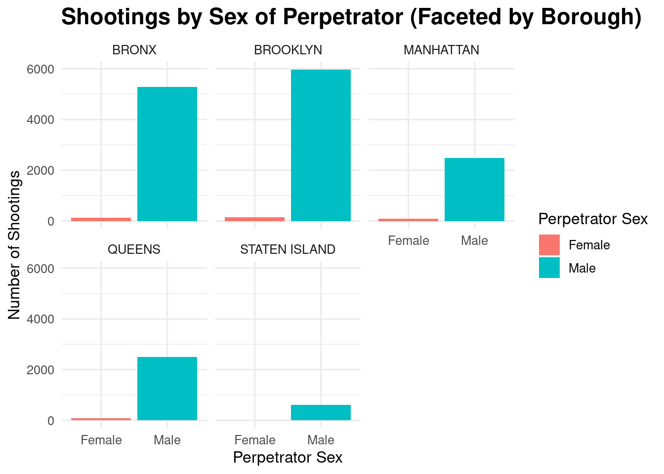
5 Staten Island 609We clean the perp_sex variable by removing missing and unavailable values. Then, we count how many shootings involved each sex in each borough. After that, we focus on male perpetrators and summarize the number of male-involved incidents by borough. The borough with the highest number of male perpetrator incidents is Brooklyn (5971 cases; 35.4%).
2.6 Tables & Graphs
2.6.1 Table (kable)
Now that we have an overview of our data, we create a table to neatly display a portion of the cleaned dataset.
# Filter out missing or unavailable perpetrator sex values
shooting_top <- shooting_clean %>% filter(!is.na(perp_sex), !(perp_sex %in% c("U","(null)"))) %>%
   # Convert occur_date to a Date format
  mutate(occur_date = lubridate::mdy(occur_date),

          # Recode perpetrator sex labels for readability
         perp_sex = case_when(
  perp_sex == "M" ~ "Male",
  perp_sex == "F" ~ "Female",
  TRUE ~ perp_sex)) %>%
  arrange(desc(occur_date)) %>%

   # Select key columns using base R indexing and display the first 10 rows
  .[, c("occur_date", "boro", "time_of_day", "perp_sex", "perp_race")] %>%
dplyr::slice_head(n = 10)

# Display the cleaned preview table
shooting_top
# A tibble: 10 × 5
occur_date boro time_of_day perp_sex perp_race
<date> <chr> <chr> <chr> <chr>
1 2024-12-31 BROOKLYN Night Male BLACK
2 2024-12-31 BROOKLYN Night Male BLACK
3 2024-12-30 BRONX Afternoon Male BLACK
4 2024-12-30 BROOKLYN Night Male BLACK
5 2024-12-30 BRONX Night Male BLACK
6 2024-12-29 BRONX Afternoon Male BLACK
7 2024-12-28 MANHATTAN Morning Male BLACK
8 2024-12-28 MANHATTAN Morning Female BLACK
9 2024-12-27 BRONX Night Male BLACK HISPANIC
10 2024-12-27 BRONX Night Male BLACK HISPANIC# Identify the most common perpetrator sex in the dataset
top_sex <- shooting_top %>% count(perp_sex, sort = TRUE) %>% slice(1)
# Create a kable table
knitr::kable(shooting_top) | occur_date | boro | time_of_day | perp_sex | perp_race |
|---|---|---|---|---|
| 2024-12-31 | BROOKLYN | Night | Male | BLACK |
| 2024-12-31 | BROOKLYN | Night | Male | BLACK |
| 2024-12-30 | BRONX | Afternoon | Male | BLACK |
| 2024-12-30 | BROOKLYN | Night | Male | BLACK |
| 2024-12-30 | BRONX | Night | Male | BLACK |
| 2024-12-29 | BRONX | Afternoon | Male | BLACK |
| 2024-12-28 | MANHATTAN | Morning | Male | BLACK |
| 2024-12-28 | MANHATTAN | Morning | Female | BLACK |
| 2024-12-27 | BRONX | Night | Male | BLACK HISPANIC |
| 2024-12-27 | BRONX | Night | Male | BLACK HISPANIC |
We remove rows with missing or unavailable perpetrator sex values, convert occur_date to a date format without the time stamp, and recode sex labels to ‘Male’ and ‘Female’ for readability. We then select key columns and display the first 10 rows of the cleaned dataset. The most common perpetrator sex in this subset is Male.
2.6.2 Graphs (ggplot2)
2.6.2.1 Time of Day Plot
To better understand patterns in the data, we visualize shooting counts by time of day using a bar chart.
shooting_time<- shooting_clean %>%
  group_by(time_of_day,boro) %>%
  summarize(total=n())
`summarise()` has grouped output by 'time_of_day'. You can override using the
`.groups` argument.ggplot(shooting_time, aes(x = time_of_day, y = total, fill = time_of_day)) +
geom_col() +
labs(title = "Time of Shootings in NYC",
x = "Time of Day", y = "Number of Shootings",fill="Time of Day") +
theme_minimal(base_size = 12) +
theme(plot.title = element_text(size = 17, family = "Georgia", face = "bold"),
axis.title.x = element_text(size = 12, family = "Georgia"),
axis.title.y = element_text(size = 12, family = "Georgia"))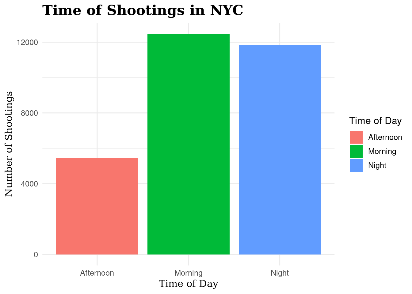
Interpretation:
We group shootings by time of day and borough, count the number of incidents, and create a bar chart showing total shootings by time of day. The fewest shooting incidents occur during the Afternoon.
2.6.2.2 Sex of Perpetrator Plot
Next, we visualize the number of shooting incidents by perpetrator sex across boroughs using a faceted bar chart.
shooting_clean_perp_sex<- shooting_clean_sex %>%
  group_by(perp_sex,boro) %>%
  summarize(total=n())
`summarise()` has grouped output by 'perp_sex'. You can override using the
`.groups` argument.shooting_clean_perp_sex <- shooting_clean_perp_sex %>%
mutate(
perp_sex = factor(perp_sex, levels = c("F","M"),
labels = c("Female","Male")))
ggplot(shooting_clean_perp_sex, aes(x = perp_sex, y = total, fill = perp_sex)) +
geom_col() +
facet_wrap(~ boro) +
labs(
title = "Shootings by Sex of Perpetrator (Faceted by Borough)",
x = "Perpetrator Sex", y = "Number of Shootings", fill = "Perpetrator Sex"
) +
theme_minimal(base_size = 12) +
theme(
plot.title = element_text(size = 17, family = "sans", face = "bold"),
axis.title.x = element_text(size = 12, family = "sans"),
axis.title.y = element_text(size = 12, family = "sans")
)
Interpretation:
We group the data by perpetrator sex and borough, count incidents, and recode sex labels to ‘Female’ and ‘Male.’ We then plot a faceted bar chart showing shootings by perpetrator sex for each borough. The borough with the fewest shootings is STATEN ISLAND (624 incidents).
2.7 Reflection
Learning how to create an R Markdown document will be very helpful when I begin working with my thesis dataset. It allows me to keep my code and explanations organized in a clear, step-by-step workflow, making it easy to see how each part of the analysis was carried out. When I return to the project later, the document serves as a built-in guide that helps me understand my previous decisions and continue the work without confusion. This structure also supports reproducibility and makes it easy to share my workflow with others.